Continuous Improvement of Analytical Methods: A framework
Chapter 1. Introduction
Regulated industries often struggle with improving their validated analytical methods. These methods are often viewed as final and untouchable. A method might pass development and validation criteria with flying colors, but in practice, it turns out to be inefficient, confusing, and leads to high rework due to frequent laboratory errors or OOS results. You feel stuck with the method because improving or changing it feels too difficult or costly.
In the pharmaceutical industry, method development and validation are based on the ICH harmonized guidelines: Q14 on analytical procedure development and Q2 on validation of analytical procedures. This article focuses on analytical methods based on these guidelines. However, the basic Lean principles presented here apply to the majority of development and validation methodologies available.
Recent years have provided a paradigm shift in how the pharmaceutical industry thinks about analytical methods due to the recent updates to ICH Q2(R2) in 2023 and ICH Q14 in 2024. The regulatory landscape has evolved from viewing methods as something final to a mindset based on a risk-based lifecycle management approach. This type of thinking requires better communication between stakeholders; you must understand your product, your manufacturing process, and your quality control.
In this article, we focus on two perspectives:
Systems thinking: Viewing your analytical method not as a standalone test, but as a critical part of a larger value stream to ensure patient safety.
Lean thinking: How to utilize Lean principles to decide what to improve, how to identify the waste in your current analytical method, and how to systematically eliminate it.
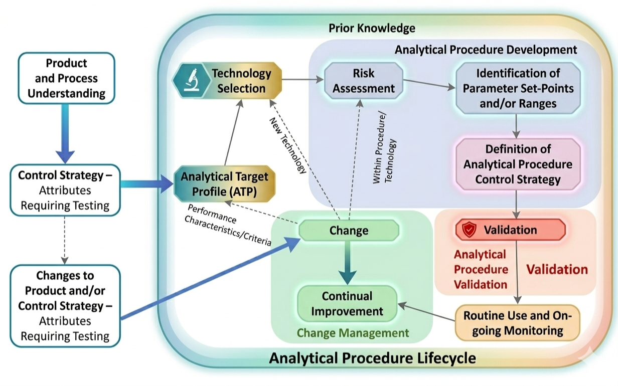
The new and updated ICH guidelines align perfectly with Lean principles. Just think of the typical process improvement framework of PDCA (Plan-Do-Check-Act). The development of your method in Q14 focuses on the Planning and Doing. Q2(R2) focuses on Checking the validity of your method. All of this is integrated with ongoing monitoring of your method using appropriate system suitability and process monitoring parameters to see trends before they become issues. You can then follow your typical change management procedure to Act and change the method while controlling risks identified during your method development risk assessment.
Together, all of this translates into the importance of systems thinking, or analytical procedure lifecycle management, as described in Q14:
To improve a method, you must first understand its purpose. In Chapter 2, we’ll define what value looks like in the lab and why knowing your process is the foundation of any successful change.
Chapter 2. Define Value
Let’s begin by first defining what value is. In a laboratory setting, the customer can be defined as the patient (or the hospital). And what delivers value to your customer? A reliable answer about whether your pharmaceutical product is safe and effective.
ICH Q14 helps the analytical scientists deliver this value via the Analytical Target Profile (ATP). It summarizes the performance characteristics of your method that must be delivered to ensure product quality. You can think of ATP as the specification of your method, which must be met.
Let’s use an HPLC assay method measuring the active ingredient in a tablet as an example. Your ATP might state your major performance characteristics as follows:
Working range: 70-130 % of nominal sample concentration
Specificity: the method must distinguish the API from impurities and degradation products with a resolution of > 2.0
Accuracy: mean recovery of 98.0–102.0% of the true value across the working range
Repeatability: RSD ≤ 1.0% (n = 6, at 100% nominal concentration)
Intermediate precision: RSD ≤ 2.0% across analysts, days, and instruments
Linearity: r² ≥ 0.999 across the range of 70–130%
These characteristics define the performance that the method you are developing must meet. It does not specify how you reach these characteristics. You might think of these characteristics as limitations, but actually they provide you with various alternatives. Down the line, if you find better alternatives to reach these characteristics, you can improve your method as long as these criteria are met!
Next, let’s define the value of your method. One technique to use is Value Stream Mapping (VSM). It is a Lean tool for drawing the full path your product or sample takes from start to finish. The point isn’t to only document the process, but it’s to make the flow of value visible. With VSM, you can see where there is waste. A good VSM separates the steps that create value from steps that simply consume your time and resources. With your HPLC assay, the value chain might include steps such as sample arrival, sample preparation, sequence setup, equipment run time, chromatogram integration, review of data and approval of data.
Everything in the map you have just created that doesn’t help you generate value is Muda (waste in Lean terms). What could be Muda in your analytical method? Here are eight categories and examples:
Waiting: Sample preparation is complete, but you have a line of analysts waiting for their turn to use your single HPLC instrument.
Defects: The system suitability of your method fails because the repeatability is 1.1% instead of 1.0% due to a poorly developed analytical method that barely met your ATP during method development and validation.
Overprocessing: Your integration parameters are suboptimal, because the analytical scientists didn't optimize them during method development. Every chromatogram requires the baseline and peak start/stops to be adjusted by hand.
Motion and transport: The analyst prints the result from the CDS, delivers it to the chemist for review, and archives the paper documents after approval. The data already exists in a validated system, but it is moved by hand between systems, which adds effort, delay, and the risk of a transcription error that triggers an investigation.
Inventory: The analytical method you are using is notoriously unreliable, which is why you run extra standards in every run just in case.
Overproduction: You test more samples, or test them more often, than the decision actually requires. Extra replicate injections are added to a sequence beyond what the ATP requires. The lab is generating data nobody will use to make a decision.
Non-utilized talent: Your experienced specialist spends their day running routine release sequences and re-integrating chromatograms instead of improving processes and leading complicated OOS investigations.
Extra processing steps: The procedure requires a manual dilution series that a single calibrated dispenser could perform in one step. A second-person review is required on every chromatogram, even those from a fully qualified, locked integration method. Each step was added for a good reason at some point, but no one has asked recently whether the reason still applies.
In conclusion, ATP tells you what provides value in your analytical method. The VSM shows you where the value is. The Muda reveals the waste in between the value. In an optimal world, your laboratory might have unlimited resources to develop, validate and improve your existing methods. However, in reality, you are always fighting for the necessary resources and need to choose your battles.
In chapter 3, we will be discussing just that: how you choose what methods to improve.
Chapter 3. Choose your battle
Not everything can be improved or fixed at once. Your QC laboratory likely has dozens or more of validated methods and every one of them has some sources of waste in them somewhere. If you try to fix them all, you’ll end up with a confusing mess with little overall impact on your laboratory performance. That is why the first decision must be what to improve first.
The Pareto principle can act as a good rule of thumb here: with most systems or analytical methods, roughly 80 % of the problems come from 20 % of the causes. A Pareto chart can help you visualize this. In short, you count the occurrences of a problem, sort them from largest to smallest, and you focus on the bars to the left. Everything else is noise.
To draw a Pareto chart, you need data. The source of data can vary, but it can be OOS investigation records, deviation reports, reruns, rework, change controls. This all depends on the priorities of your laboratory leadership. The top priority of your laboratory might be the reduction of OOS investigations by 30 %, the elimination of reruns by 50 %, or the reduction of analysis costs by 30 % through method optimization. The sky is the limit!
Let’s illustrate this by drawing a Pareto chart using OOS investigations across an imaginary QC laboratory:
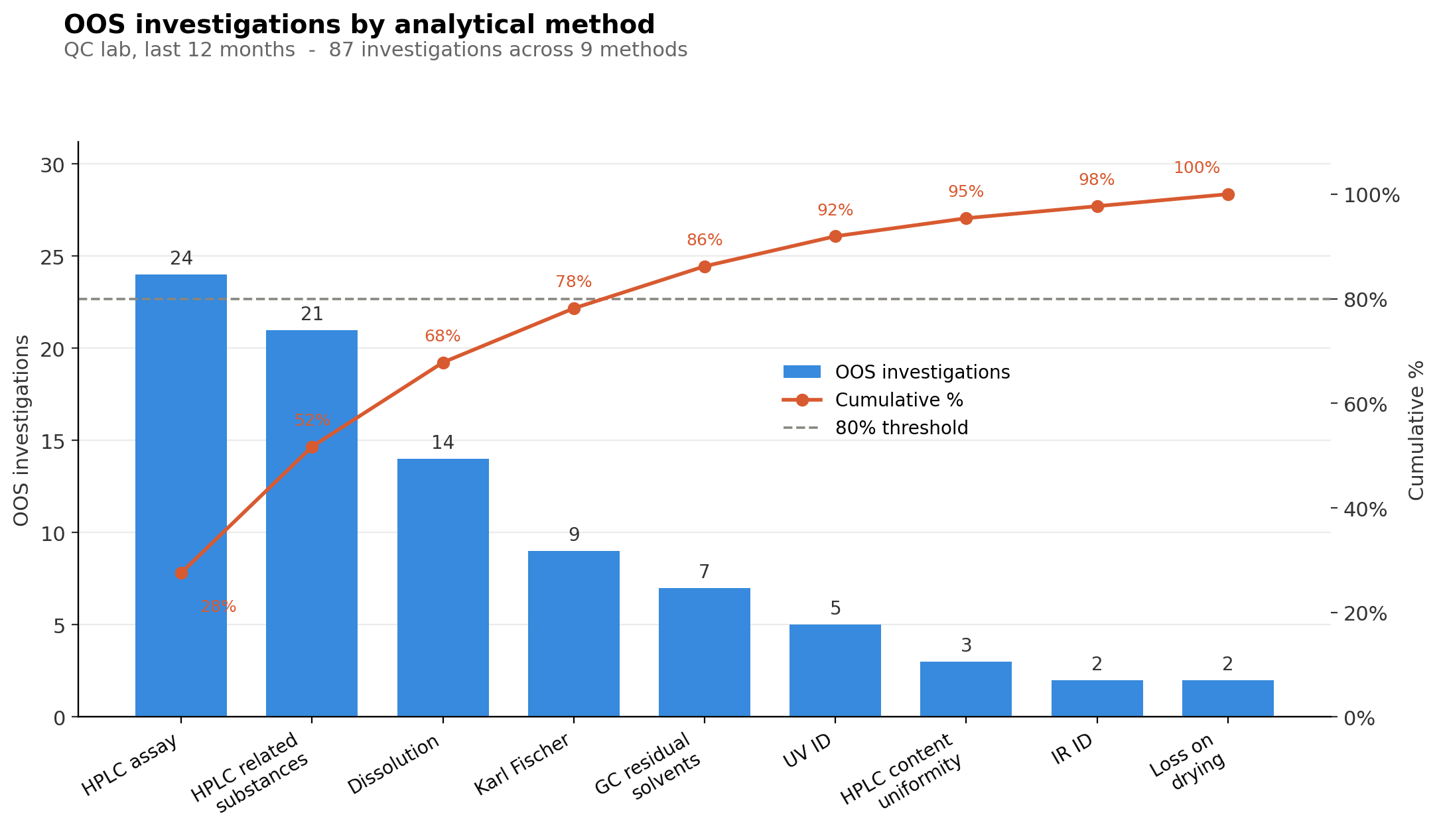
From this chart, you can clearly see that the two biggest sources of OOS investigations are HPLC assay and HPLC related-substances methods (e.g. impurities and degradation products). Based on the Pareto principle, the biggest gains for your laboratory would come from focusing on these two method types. By doing this, you will make the most progress toward your laboratory goal (in this exercise, our goal is to reduce the prevalence of OOS investigations by 30 %). For the sake of this example, let's focus on just the HPLC assay method. The Pareto principle only shows you the symptoms, not the causes themselves.
Next, we would focus on digging through the different OOS investigations to find trends. We can use the Pareto principle for this as well:
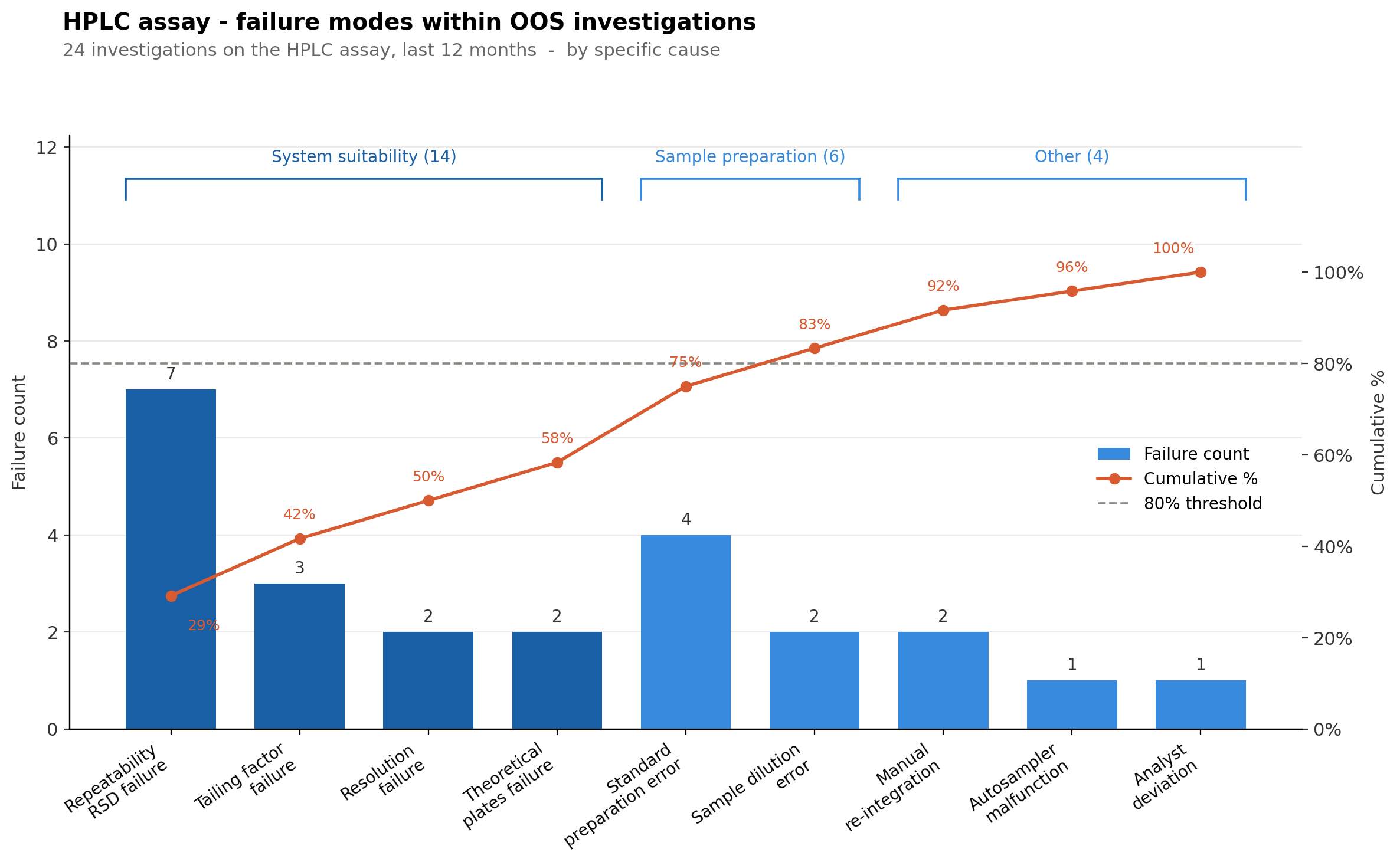
Our further data analysis indicated three distinct categories of OOS investigations: system suitability, sample preparation and other miscellaneous events. From the failure counts, we see clearly that system suitability is the biggest culprit, with the following identified causes:
Repeatability (RSD%) failures
Tailing factor failures
Resolution failures
Theoretical plates failures
All of these failures could be caused by a number of things. It’s likely you need to perform further root cause analysis to fully lock on a possible solution. Next, we perform a workshop (Kaizen event) with various laboratory experts to fully confirm the root cause and discover where we should be focusing our improvement efforts. The end result of this workshop is the following Ishikawa diagram:
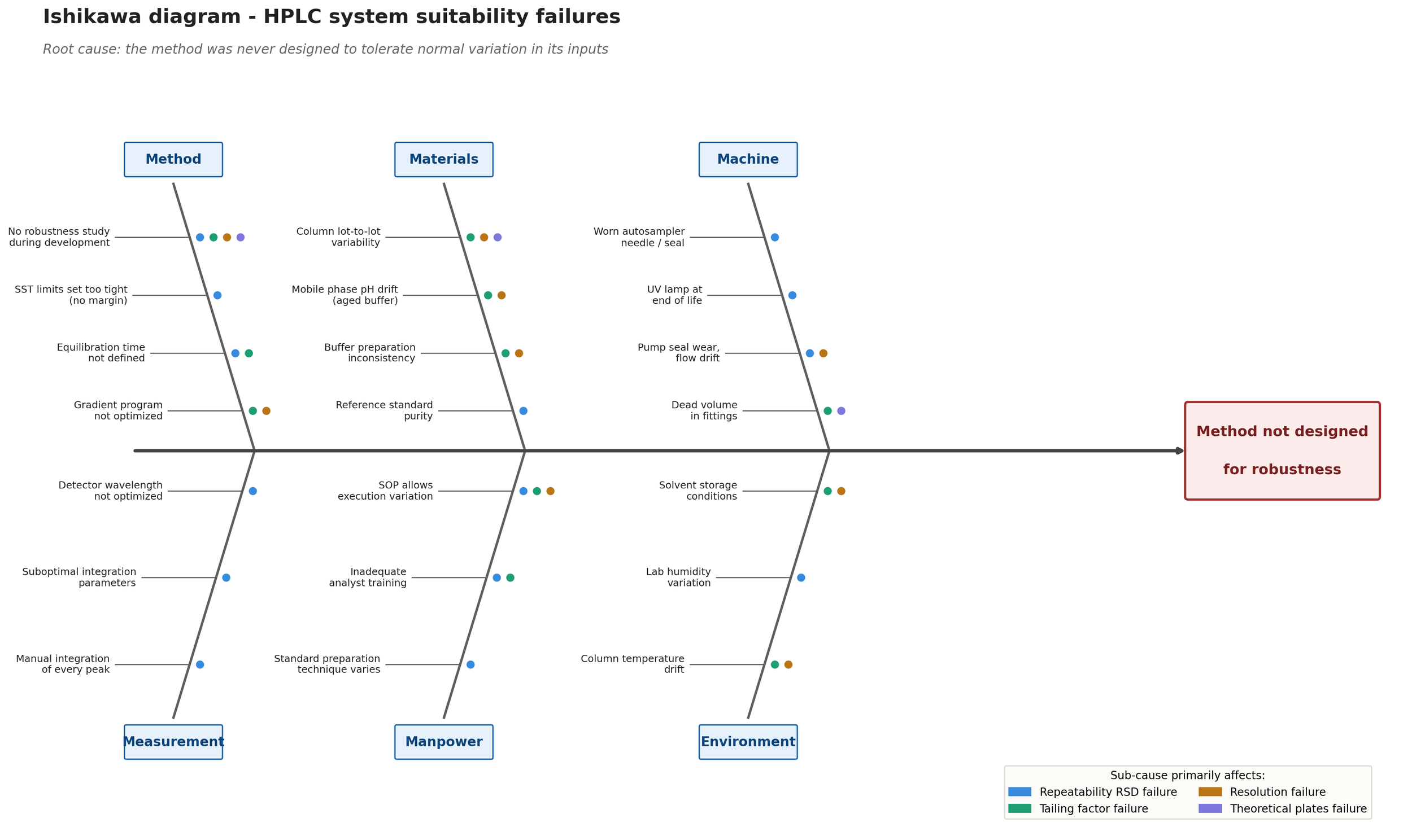
As we can summarize from the Ishikawa diagram, culprit is insufficient method development before validation and transfer to routine use in the QC laboratory. The method development likely failed to account for method drift during the method lifecycle, leading into multiple OOS investigations down the line. This can only be fixed by returning back to the drawing board and fixing the method itself by tighter controls for the variables that matter.
Because the actual root cause traces back to the method development, we will next focus on designing your method for robustness by utilizing ICH Q14 enhanced approach.
Chapter 4. Design for Robustness
We successfully identified a single root cause for your HPLC assay method: the method in question was never designed to account for normal process variation. Retention times shifting between runs. Resolution drifts with column aging. Sample preparation protocol introduces variability due to different analysts having different pipetting techniques. All these examples point at a single critical flaw: the robustness of the method itself. That is why we are next focusing on designing your method for robustness. Ideally, this should be done during initial method design. Revalidation in pharma is costly and time-consuming, which is itself a form of Muda that good design prevents.
Lean has a name for this kind of design practice: poka-yoke, or mistake-proofing. The basic idea is to build quality into the process to prevent the occurrence of the error or to help detect the error before it becomes an issue, such as an OOS investigation. A well developed method is built to withstand regular process variation that will inevitably happen during routine use.
ICH Q14 uses the term enhanced approach to analytical development. In regular, simplified method development, you’re simply asking for the method to meet the acceptance criteria in validation once. With the enhanced approach, you’re testing the validation acceptance criteria across a range of conditions to see how capable the method is in routine use. To put it simply: the traditional approach produces a method that passes validation once. The enhanced approach produces a method that keeps passing validation criteria during the entire method lifecycle.
What are the tools to get there, then?
Two practical tools are introduced in ICH Q14: Design of Experiments (DOE) and Method Operable Design Region (MODR). In the context of analytical method development, DOE can be defined as a defining and testing philosophy where several method parameters are varied at once with a carefully designed experiment: mobile phase composition, column temperature, pH, flow rate. The idea is to understand how each one of these parameters and combinations of them, affects the performance of the method.
Traditionally, many chemists are taught that in science, you must only vary one parameter at once. However, this type of outdated thinking will lead to suboptimal methods. By teaching your chemists the importance of statistics and DOE, your laboratory will develop better methods with less time spent when the alternative is to vary conditions one parameter at a time.
The use of DOE in designing analytical methods also links well with the philosophy of MODR. With the use of DOE and MODR, you will identify a region of safe parameters where the method reliably keeps meeting the ATP performance criteria. Inside MODR, your method keeps working. This is crucial to understand because your method will experience drift during routine use.
DOE and MODR are complex topics and their thorough use is not in the scope of this introductory article. However, to better illustrate the point I’m trying to make, let’s look at an example:
You're developing the HPLC assay from Chapter 2. The ATP requires a resolution of ≥ 2.0 between the active and its nearest degradant, and a repeatability RSD of ≤ 1.0%. The traditional approach would test each parameter in isolation. This might include changing the mobile phase organic content from 38 % to 42 % while holding all other parameters fixed. Your experiment might produce the best resolution of 2.1 with 40 % organic content, so you can safely lock that in. Then you perform the same experiment with pH. In the end you find that the best set of conditions are 40 % organic phase, 30 °C column temperature and pH of 3.0.
However, with DOE, you use a structured design (a small factorial or response surface study) that varies multiple conditions at the same time while judging the result against your ATP performance criteria. With this type of design, you will find the hidden interactions. You discover that the organic content and column temperature actually interact with each other. At 30 °C, your method meets the ATP criteria of 2.0 with ease while varying the organic content from 38 to 42 %. At 35 °C, your resolution falls below 2.0 as soon as the organic content drops below 40 %. This is the interaction you will miss when only testing one criterion at a time.
This is where MODR comes in.
With the enhanced approach in ICH Q14, you discover the parameter conditions where your method keeps meeting the ATP performance criteria. In our example, the MODR might be as follows:
Mobile phase organic content 38 - 42 %
Column temperature 28 - 32 ° C
Buffer pH 2.9 - 3.1
Inside this range of parameters, your method will keep working. Outside this range, your resolution or your RSD% might be insufficient. When you design your method around MODR, you can actually use this MODR in your regulatory submission when you follow ICH Q14 and ICH Q2(R2). You can even write this MODR into your SOP, and it will give you the freedom to make small adjustments later due to method drift, normal process variation, and OOS investigations.
Where is the value in this?
Fewer system suitability failures: your method is designed to withstand normal variation in routine use.
Fewer OOS investigations: Your method parameters can be varied across the MODR to prevent drift where your method performance is insufficient.
Faster troubleshooting: Due to better robustness testing, you already understand how all the critical parameters affect the method performance and how they interact together.
Regulatory benefits: Small adjustments inside MODR are justified by your method development data. This data will help you justify any relevant minor changes to the method.
Easier changes down the line: Changing columns, instruments, or acceptance criteria is easier because you already have data to compare the changes against.
Less waste in the laboratory: With quality built into your method, you avoid the Muda introduced in chapter 2.
In chapter 5, we will look into more details on how to manage your method lifecycle and ensure continuous improvement of your analytical methods is possible.
Chapter 5. Lifecycle Management and continuous improvement
Let’s imagine we have designed a robust method capable of meeting the ATP performance criteria. The next step is to implement the method into your QC laboratory.
In ICH Q14, the concept of Analytical Procedure Lifecycle Management (APLM) is introduced. The idea is to integrate all the stages of your method lifecycle into one. This includes development, validation, routine monitoring and change management of the method. These steps are no longer separate, but they are a part of the system.
This is where systems thinking introduced in chapter 1 comes in. You have set your ATP in chapter 2. You have defined the operating range of yout method with MODR in chapter 4. Next, with APLM, you provide the framework on how to ensure you keep within this range and improve your method as needed.
Your best tool to achieve this is to use statistics. For this, a simple control chart might be sufficient.
Let’s continue our OOS investigation example from chapter 3. This time, we have defined a MODR our method can operate in. To fully utilize the capabilities of ICH Q14, we could use control charts to plot the system suitability parameters directly from our Chromatography Data System (CDS). Of course, while this is optimal to reduce manual labor, you could simply utilize Excel to do the same.
As the Pareto charts showed us in chapter 3, system suitability failures were the biggest source of OOS investigations for our HPLC assay method. We create a control chart of standard RSD%, tailing factor, resolution and theoretical plates (pro tip: tracking every parameter might be Muda in itself. Pick the one(s) that has the highest impact for your method. For this, your expert judgement is needed).
By utilizing control charts in this manner, you can see trends before they become issues and potentially greatly reduce the number of OOS investigations. If done well, control charts support poka-yoke at the method lifecycle level.
Below, you can see an example of what this might look like in your laboratory:
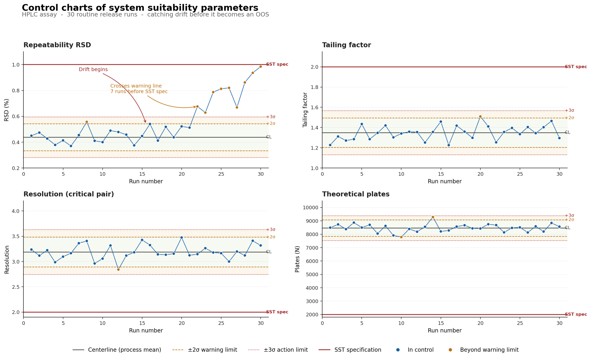
In the example above, you can see control charts of four system suitability parameters across 30 routine release runs of the HPLC assay. Tailing factor, resolution, and theoretical plates remain in control. Repeatability RSD begins drifting at run 15 and crosses the +2σ warning limit at run 22. This is several runs before our system suitability acceptance criteria are exceeded, which would trigger an OOS investigation.
In a QC laboratory well-versed in statistics, this would raise the alarm bells well before your analysis results are affected. Your chemists could then come up with solutions and ensure the method performance drift doesn't become an actual issue. After all, when your process variation exceeds 3 sigma, something has changed in your method. This is because roughly 99.7 % of measurements in a stable process are within ±3 sigma of the mean, so any trends outside this range are very likely due to a real issue, not just noise (assuming your data is normally distributed).
This is the value of using statistics in routine use.
Next, let's imagine we have our control charts up and we detect a drift in our method. What's next? Broadly, you have two paths, and the difference between them is where the regulatory framework starts to matter.
Option 1: adjustment within the MODR. The change stays inside the approved design space (say, shifting mobile phase organic content from 40 % to 41 %). Under ICH Q14 chapter 5, movements within the approved MODR do not require regulatory notification, assuming ICH Q12 is implemented in the markets your product is sold in. Operationally, this could be a documented change in your QMS, verified by system suitability with the new conditions, and added in your working instructions and control chart, and then implemented into routine monitoring.
Option 2: change to the MODR. Unforeseen drift forces you to tighten or extend the approved range of parameters. This is a change to an Established Condition (EC) and triggers a lot more work: a risk assessment under ICH Q9, supporting data to demonstrate the ATP is still met (possibly a new DOE), regional categorization of the change, a variation submission, and implementation only after approval. Once approved, you update your control strategy and resume monitoring.
With a well-defined process for method lifecycle management, you keep your workload acceptable even under Option 2. But the reality is more complicated than the framework suggests. This article assumes regulators have implemented ICH Q14 and ICH Q12, and in practice, there are still non-ICH countries that operate under traditional change frameworks. For a global product, a single MODR change might require several submission types. This shouldn't discourage you. A well-designed method with a suitable MODR pays off, because your OOS investigations are fewer, there is less waste in your laboratory, and routine operations are much simpler.
Please work together with the necessary stakeholders in your organization to always ensure you're going by the book. My recommendation is to build standard processes into your quality system that actually support continuous improvement of your analytical methods.
To summarize, the ICH guidelines give you the framework for implementing method lifecycle management, and Lean gives you the practical tools to actually improve your methods. While this article focused on QC laboratory applications in the pharmaceutical industry, the Lean principles introduced here apply to any laboratory with rigorous quality systems. You should always aim to reduce Muda and build quality into your processes.
Sources
[1] International Council for Harmonisation of Technical Requirements for Pharmaceuticals for Human Use (ICH) (2024) ICH Q14 Guideline on analytical procedure development. Distributed by the European Medicines Agency. Available at: https://www.ema.europa.eu/en/documents/scientific-guideline/ich-q14-guideline-analytical-procedure-development-step-5-revision-1_en.pdf. (Accessed:19.04.2026)
[2] International Council for Harmonisation of Technical Requirements for Pharmaceuticals for Human Use (ICH) (2023) ICH Q2(R2) Guideline on validation of analytical procedures. Available at: https://database.ich.org/sites/default/files/ICH_Q2(R2)_Guideline_2023_1130.pdf. (Accessed: 19.04.2026)
[3] International Council for Harmonisation, 2023. ICH Harmonised Guideline: Quality Risk Management Q9(R1). Final version, adopted 18 January 2023. Geneva: ICH. Available at: https://database.ich.org/sites/default/files/ICH_Q9(R1)_Guideline_Step4_2022_1219.pdf. (Accessed: 19.05.2026)
[4] International Council for Harmonisation, 2019. ICH Harmonised Guideline: Technical and Regulatory Considerations for Pharmaceutical Product Lifecycle Management Q12. Final version, adopted 20 November 2019. Geneva: ICH. Available at https://database.ich.org/sites/default/files/Q12_Guideline_Step4_2019_1119.pdf. (Accessed:19.05.2026)
Illustrations and graphs shown in this article were generated with ChatGPT and Gemini 3.1 Pro.